Physics Derivation Graph navigation Sign in

Recommendation: Read the user documentation and FAQ first. This page assumes familiarity with the jargon used in the Physics Derivation Graph.

This page provides background context for design decisions associated with the Physics Derivation Graph (PDG). Contributions to the project are welcome; see CONTRIBUTING.md on how to get started. The Physics Derivation Graph is covered by the Creative Commons Attribution 4.0 International License, so if you don't like a choice that was made you are welcome to fork the Physics Derivation Graph project.

Contents

  1. Design Decisions
  2. Grammar of the controlled natural language
  3. Numeric indices are the core enabling concept for the PDG
  4. Data structure used in the PDG
  5. \(\rm\LaTeX\) representation of expressions
  6. Derivation to Graph from First Principles
  7. Historical design evolution
    1. Other approaches
      1. Networkx
      2. GraphML
      3. RDF/OWL
  8. Comparison of Syntax Options
    1. Test Cases
    2. Quantitative Comparison of Test Cases
    3. Qualitative Comparisons of Syntax Methods
    4. Transforming between Syntax options
    5. Auditing the Correctness of Derivations
  9. [Appendix] Comparison of Computer Algebra Systems
    1. Sage
    2. Mathematica
    3. Sympy
    4. HOL Light theorem prover
  10. [Appendix] Outside of Current Scope


Design Decisions

The objective for the Physics Derivation Graph project is to write down all known mathematical physics in a way that can be both read by humans and checked by a computer algebra system. To do that, primary design considerations include how to represent the objects (e.g., inference rules and expressions and symbols) and what data structure is sufficient for the objective.

This page describes the current status and historical evoluation of design decisions critical to the Physics Derivation Graph.


Grammar of the controlled natural language

In the Physics Derivation Graph, the primary vocabulary is a set of inference rules that relate mathematical expressions.
The grammar of the Physics Derivation Graph is specified by this list, with all items joined by "and":

The full list of vocabulary used in the Physics Derivation Graph is documented in the list of inference rules and list of expressions and list of symbols.


Numeric indices are the core enabling concept for the Physics Derivation Graph

The visualization of a graph with expressions and inference rules as nodes relies on each node having a distinct index. Each expression, symbol, and inference rule appears only once in the database. This is made possible through use of unique IDs associated with every facet of the visualization. To see what this means in terms of the "period and frequency" example on the homepage, here is a view of the indices supporting that visualization for two sequential steps:


Figure 1. Two steps with all numeric IDs shown.

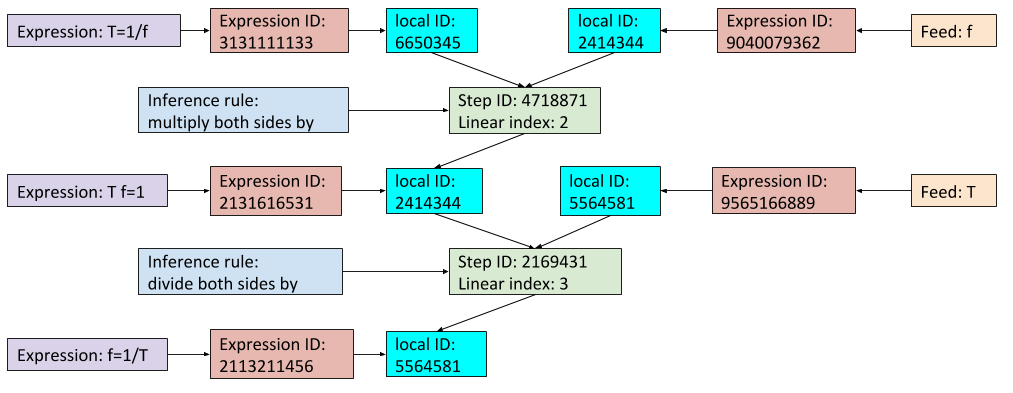
Manipulating these indices underlies all other tasks in the Physics Derivation Graph. Access to these indices is performed through a single data structure.


Data structure used in the Physics Derivation Graph

The Physics Derivation Graph is currently stored in a single JSON file. The JSON file is read into Python as a dictionary.

JSON is convenient because it is plain text and the ease of detailed validation available using schemas. The many alternatives to JSON (e.g., SQLite, Redis, Python Pickle, CSV, GraphML) offer trade-offs, a few of which have been explored.


\(\rm\LaTeX\) representation of expressions

There are multiple choices of how to represent a mathematical expression. The choices feature trade-offs between conciseness, ability to express the range of notations necessary for Physics, symantic meaning, and ability to use the expression in a computer algebra system (CAS). See the comparison of syntax below. \(\rm\LaTeX\) was selected primarily because of the common use in Physics, display of complex math, conciseness, and expressiveness. The use of \(\rm\LaTeX\) means other tasks like parsing symbols and resolving ambiguity are harder.


Derivation of Graph from First Principles

A reasonable question is, "Why is the Physics Derivation Graph complicated?" To answer that, let's walk through the process of tracking information used in a derivation.

A simple derivation is the transition from the expression \(T = 1/f\) to \(f = 1/T\), the same example used on the home page. The purpose of this section is to explain how a graph relates to the steps associated with this math.

The steps needed to make the transformation are to multiply both sides by \(f\), then divide both sides by \(T\). There are four steps in this derivation:

  1. declare initial expression \(T=1/f\)
  2. multiply both sides of \(T=1/f\) by \(f\) to get \(T*f=1\)
  3. divide both sides of \(T f=1\) by \(T\) to get \(f=1/T\)
  4. declare final expression: \(f=1/T\)
This expansion to atomic steps is not typically documented. This expansion can be tedious for derivations, but it is necessary for validation of steps using a Computer Algebra System. As a recommendation, starting the derivation on paper and then expanding to atomic steps with inference rules is best done on paper.

The next step is to visualize this graph. When building a graph, there are three types of nodes: inference rules, expressions, and feeds. The graph will only have three types of directed edges:

Although there is enough information present to generate a graph, the objective for the Physics Derivation Graph is to support more complex derivations and to link multiple derivations. In the Physics Derivation Graph the inference rule "multiply both sides by" may appear in multiple steps. The graph should not render multiple uses of the same inference rule as the same node. Multiple references to the same expression should be a single node. Therefore, an index which has a scope limited to the local derivation step is needed. This leads to the notion of a unique numeric index local to each inference rule. The local index for the inference rule is a unique identifier within a derivation step.

Another complication arises regarding the expressions. The usefulness of \(T = 1/f\) depends on what is reading the expression. Multiple readers of the expression can be expected: humans, LaTeX, and Computer Algebra Systems (e.g., Mathematica, Sympy). This leads to the need for a unique identifier which is associated with the expression independent of the representation. In Logic, this unique identifier is referred to as the Godel number. Similarly, the "feeds" (here f and T need unique identifiers.

To summarize the above points,

The expression index is the same across all derivations, whereas the local index is scoped to just the derivation step. Similarly, the inference rule index is specific to the derivation step.

The inference rule needs the local index to build the graph. The expression needs a local index to build the \(\rm\LaTeX\) PDF.

In addition to the inference rules and expressions, each \(\rm\LaTeX\) expression actually represents an Abstract Syntax Tree (AST) composed of symbols.


Figure 4. All of the jargon used and the relation between jargon used in the Physics Derivation Graph.


Historical design evolution

The Physics Derivation Graph has progressed through multiple architectures, with data structure changes keeping pace with the developer's knowledge.

  1. plain text: databases for comments, connections, equations, operators. Perl script to convert database content to images. One line per entry in each database.
  2. XML:
  3. CSV:
  4. file per expression:
  5. property graph: a very limited exploration. Written in Cypher/Neo4j but could also use Gremlin/TinkerPop. No significant code base. Schema:

    Schema for property graph representation.
  6. sqlite: a very limited exploration. No significant code base. Schema: TODO: is this schema in 3NF?
  7. web interface: the current implementation. Uses Python, Flask, Docker. Data is stored in a JSON file. Limited support for checking inference rules using Sympy. Storage formats evolved:
    1. nested Python dictionaries and lists stored as a Python Pickle
    2. nested Python dictionaries and lists stored as a JSON file. With this approach the schema can be validated
    3. nested Python dictionaries and lists stored as a JSON file stored in Redis. Retains the schema validation of JSON while preventing concurrent writes to file; see https://redis.io/topics/transactions
    4. nested Python dictionaries and lists stored as a JSON file stored in SQLite3. Part of the migration towards table-based implementation. SQLite3 is better than Redis because Redis requires a Redis server to be running whereas SQLite3 is a file.
Each of these have required a rewrite of the code from scratch, as well as transfer code (to move from n to n+1). The author didn't know about property graphs when implementing v1, v2, and v3.

Within a given implementation, there are design decisions with trade-offs to evaluate. Knowing all the options or consequences is not feasible until one or more are implemented. Then the inefficiencies can be observed. Knowledge gained through evolutionary iteration is expensive and takes a lot of time.

A few storage methods were considered and then rejected without a full implementation.

Other approaches

Networkx


import networkx as nx
G=nx.digraph()
G.add_edge([8332941,8482459])
G.add_edge([8482459,6822583])
G.add_edge([5749291,6822583])
G.add_edge([6822583,8341200])
G.add_edge([8341200,9483715])
G.add_edge([8837284,9483715])
G.add_edge([9483715,9380032])
G.add_edge([9380032,8345721])
nx.plot()
plt.show()

GraphML

See GraphML file format.

RDF/OWL

The Physics Derivation Graph can be expressed in RDF.

Each step in a derivation could be put in the subject–predicate–object triple form. For example, suppose the step is

Input 1: y=mx+b
inference rule: multiply both sides by
feed: 2
output 2: 2*y = 2*m*x + 2*b
Putting this in RDF,
step 1 | has input | y=mx+b
step 1 | has inference rule | multiply both sides by
step 1 | has feed | 2
step 1 | has output | 2*y = 2*m*x + 2*b
While it's easy to convert, I am unaware of the advantages of using RDF. The Physics Derivation Graph is oriented towards visualization. SPARQL is the query language for RDF. I don't see much use for querying the graph. Using RDF doesn't help with using a computer algebra system for validation of the step.


Comparison of Syntax Options

Here methods of capturing mathematical syntax required to describe derivations in physics are compared. This survey covers \(\rm\LaTeX\), Mathematical Markup Language (MathML), Mathematica, and SymPy. For MathML, both Presentation and Content forms are included.

Although \(\rm\LaTeX\) is intuitive for scientists and is concise, it is a typesetting language and not well suited for the web or use in Computer Algebra Systems (CAS). Mathematica is also concise and has wide spread use by scientists, though its cost limits accessibility. Mathematica is also proprietary, which limits the ability to explore the correctness of this CAS

\(\rm\LaTeX\) is concise and is widely used in the scientific community. It does not work well for portability to other representations and is ill-suited for use by CAS. For the initial phases of development for the Physics Derivation Graph, portability and compatibilty with a CAS are not the priority. Since getting content into the graph is the priority, the Latex representation will be used.

For this survey it is assumed that users cares about the learning curve, leveraging previous experience, how wide spread use in their community, speed, ease of input, presentation (rendering), ability to access content across devices, OS independence, ease of setup. To evaluate criteria relevant to users, including the ability to manually input syntax, the ability to transform between representations, and the ability to audit correctness.

Use of a single syntax for the graph content is important. To illustrate why, consider the approach where each syntax is used for its intended purpose -- Latex for rendering equation, SymPy for the CAS, and MathML for portability. This introduces a significant source of error when a single equation requires three distinct representation. The manual entry could result in the three representations not being sychronized. Thus, a single representation satisfying multiple criteria is needed. If no single syntax meets all the needs of the Physics Derivation Graph, then the requirements must be prioritized.

This comparison is between syntax methods which do not serve the same purpose. Latex is a type-setting language, while Mathematica and SymPy are Computer Algebra Systems (CAS). The reason these approaches for rendering and CAS were picked is twofold: they are widely used in the scientific community and they address requirements for the Physics Derivation Graph.

We can ignore syntax methods which do not support notation necessary for describing physics. Example of this include ASCII and HTML. Storage of the generated content (essentially a knowledge base for all of physics) isn't expected to exceed a Gigabyte, so compactness in terms of storage isn't a criterion in this evaluation.

Test Cases

to demonstrate the variety of uses in distinct domains of Physics, a set of test cases are provided in this section. These cases are not meant to be exhaustive of either the syntax or the scientific domain. Rather, they are examples of both capability requirements of the Physics Derivation Graph and of the syntax methods.

Case 1 is a second order polynomial. Algebra \begin{equation} a x^2 + b x + c = 0 \label{eq:polynomial_case1_body} \end{equation}

Case 2, Stokes' theorem, includes integrals, cross products, and vectors. Calculus \begin{equation} \int \int_{\sum} \vec{\nabla} \times \vec{F} \dot d\sum = \oint_{\partial \sum} \vec{F}\dot d\vec{r} \label{eq:stokes_case2_body} \end{equation}

Case 3: Tensor analysis. Einstein notation: contravariant = superscript, covariant = subscript. Used in electrodynamics \begin{equation} Y^i(X_j) = \delta^i_{\ j} \label{eq:tensor_analysis_case3_body} \end{equation}

Case 4 covers notation used in Quantum Mechanics. Symbols such as \(\hbar\) and Dirac notation are typically used.

Case 4a is the creation operator \begin{equation} \hat{a}^+ |n\rangle = \sqrt{n+1} |n+1\rangle \label{eq:creation_operator_case4a_body} \end{equation}

Case 4b is the uncertainty principle \begin{equation} \sigma_x \sigma_p \geq \frac{\hbar}{2} \label{eq:uncertainty_principle_case4b_body} \end{equation}

Case 4c: Lüders projection \begin{equation} |\psi\rangle \rightarrow \sum_n |c_n|^2 P_n,\ \rm{where}\ P_n = \sum_i |\psi_{ni}\rangle \langle \psi_{ni}| \label{eq:Luders_projection_case4c_body} \end{equation}

Quantitative Comparison of Test Cases

Name case 1 case 2 case 3 case 4a case 4b case 4c
Latex 20 101 26 45 39 110
PMathML 324 538 348 372 250
CMathML 381
Mathematica
SymPy

MathML is comprised of empty elements (symbols, e.g., <plus/>), token elements (both ASCII and entities), and annotation elements. The token elements in Presentation MathML include mi=identifiers, mn=numbers, mo=operators. The token elements in Content MathML include ci=identifiers and cn=numbers.

Character count for the MathML was carried out using

wc -m mathML_presentation_case*.xml

Qualitative Comparisons of Syntax Methods

Latex, MathML, and SymPy are free and open source. Mathematica is proprietary and not free.

For Physicists comfortable writing journal articles in Latex or exploring ideas in Mathematica, these are natural syntax methods. Both Latex and Mathematica are concise, making them intuitive to read and quick to enter. MathML is a verbose syntax which is lengthy to manually enter and yield difficult to read the native XML.

Unicode is needed to support Dirac notation and any other non-ASCII text in MathML

Transforming between Syntax options

Wolfram Research offers the ability to convert from Mathematica expressions to MathML on their site www.mathmlcentral.com/Tools/ToMathML.jsp. A CAS typically produces output syntax such as Latex or MathML in a single format. However, there are often many ways to represent the same math, equation \ref{eq:example_partial_derivative_representations}.

Auditing the Correctness of Derivations

Latex and Presentation MathML are intended for rendering equations and are not easily parsed consistently by a CAS. For example, scientists and mathematicians often render the same partial differential operation in multiple ways: \begin{equation} \frac{\partial^2}{\partial t^2}F = \frac{\partial}{\partial t}\frac{\partial F}{\partial t} = \frac{\partial^2 F}{\partial t^2} = \frac{\partial}{\partial t}\dot{F} = \frac{\partial \dot{F}}{\partial t} = \ddot{F}. \label{eq:example_partial_derivative_representations} \end{equation} All of these are equivalent.


Comparison of Computer Algebra Systems

Sage, Mathematica, and SymPy are candidates capable of checking the correctness of derivations.

Sage

The following Sage code checks that the claimed step as stated by the inference rule is carried out correctly:

T=var('T')
f=var('f')
# latex input: T = 1/f
input_expr = (1)/(f) == (T)
# latex output: T f = 1
expected_output_expr = T * f == 1
# latex feed: f
feed = f
input_expr * feed == expected_output_expr
The output is
True
which means that the claimed step in the derivation was implemented consistent with the inference rule applied.

Sage code can be run in https://sagecell.sagemath.org/.

In this analysis of Sage the support for standard operations wasn't sufficient.

Mathematica

A computer algebra system like Mathematica can validate the steps of a derivation.

Input:

multiplyBothSidesOfExpression[LHS_, relation_, RHS_, feed_] := {LHSout = LHS*feed, relationOut = relation, RHSout = RHS*feed}
divideBothSidesOfExpression[LHS_, relation_, RHS_, feed_] := {LHSout = LHS/feed, relationOut = relation, RHSout = RHS/feed}

LHS = T;
RHS = 1/f;
relation = "=";
{LHS, relation, RHS}

result = multiplyBothSidesOfExpression[LHS, relation, RHS, f]; (* should yield T*f=1 *)
result = divideBothSidesOfExpression[result[[1]], result[[2]], result[[3]], T]; (* should yield f=1/T *)

{result[[1]], result[[2]], result[[3]]}

Output:

{T,=,1/f}

{f,=,1/T}
Quadratic equation derivation
First, set up the inference rules:
dividebothsidesby[expr_, x_] := Apart[First[expr]/x] == Apart[Last[expr]/x];
subtractXfromBothSides [expr_, x_] := First[expr]-x == Last[expr]-x;
addXtoBothSides[expr_, x_] := First[expr]+x == Last[expr]+x;
subXforY[expr_, x_, y_] := expr /. x -> y
raiseBothSidesToPower[expr_, pwr_] = First[expr]^pwr == Last[expr]^pwr
simplifyLHS [expr_, condition_] := FullSimplify [First[expr], condition] == Last[expr]
Next, use the inference rules
func = a*x^2+b*x+c == 0
func = dividebothsidesby[func, a]
func = subtractXfromBothSides [func, c/a]
func = addXtoBothSides[func, (b/(2 a))^2]
func = subXforY[func, First[func], (x+b/(2 a))^2]
func = subXforY[func, Last[func], (b^2-4 ac)/(4 a^2)]
func = raiseBothSidesToPower[func, (1/2)]
func = simplifyLHS [func, (x+b/(2 a)) > 0]
func = subXforY[func, Last[func], ±Last[func]]
func = subtractXfromBothSides [func, b/(2 a)]

Sympy

The motives for using Sympy are the cost (free), the code (open source), the integration (Python), support for Physics, and the support for parsing Latex.

The snippets of SymPy can be run in http://live.sympy.org/

HOL Light theorem prover

HOL Light tutorial


Outside of Current Scope

Although the Physics Derivation Graph is intended to be comprehensive across domains, there are aspect of Physics not within the current scope of the project:

These aspects could be included if the data structure and workflow were adapted to an expanded scope.