Recommendation: Read the user documentation and FAQ first.
This page provides background context for design decisions associated with the Physics Derivation Graph (PDG). Contributions to the project are welcome; see CONTRIBUTING.md on how to get started. The Physics Derivation Graph is covered by the Creative Commons Attribution 4.0 International License, so if you don't like a choice that was made you are welcome to fork the Physics Derivation Graph project.
Looking for the API? See API documentation.
Contents
The visualization of a graph with expressions and inference rules as nodes relies on each node having a distinct index. Each expression, symbol, and inference rule appears only once in the database. This is made possible through use of numeric IDs associated with every facet of the visualization. To see what this means in terms of the "period and frequency" example on the homepage, here is a view of the indices supporting that visualization for a single step:
Manipulating these indices underlies all other tasks in the Physics Derivation Graph. Access to these indices is performed through a single data structure.
The Physics Derivation Graph is currently stored in a single JSON file. The JSON file is read into Python as a dictionary.
JSON is convenient because it is plain text and the ease of detailed validation available using schemas. The many alternatives to JSON (e.g., SQLite, Redis, Python Pickle, CSV, GraphML) offer trade-offs, a few of which have been explored.
There are multiple choices of how to represent a mathematical expression. The choices feature trade-offs between conciseness, ability to express the range of notations necessary for Physics, symantic meaning, and ability to use the expression in a computer algebra system (CAS). See the comparison of syntax below. \(\rm\LaTeX\) was selected primarily because of the common use in Physics, display of complex math, conciseness, and expressiveness. The use of \(\rm\LaTeX\) means other tasks like parsing symbols and resolving ambiguity are harder.
The complexity supporting a technology is proportional to the number of abstraction layers required to enable it.
Python as a "glue" language is leveraged to connect existing tools like \(\rm\LaTeX\), Flask, logging, manipulation of data. Also, Python is the language the project owner is most comfortable with. And it is free and open source.
Python libraries: matplotlib, black, mypy, pycallgraph, gunicorn, prospector, pandas, jsonschema, sympy, antlr4-python3-runtime, flask-wft, graphviz
The model-view-controller (MVC) is a way to separate presentation from the backend computation and data transformation.
Note on using MVC with Flask and WTForms: For webpages with forms, the form submission should return to controller.py rather than linking to next page.
Containerization provides documentation of software dependencies and shows the installation process, enabling reproducibility and platform independence.
Alpine was investigated as a candidate OS but was found to be insufficient. Ubuntu provides necessary packages.
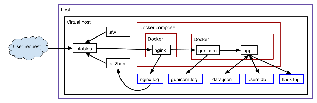
To provide a web interface, Flask is used. HTML (with Javascript) pages are rendered using Jinja2. Mathematical expressions rely on MathJax Javascript. Flask is not intended for production use in serving Python applications, so Gunicorn is the Web Server Gateway Interface. Nginx provides an HTTP proxy server.
Why this complexity is relevant is addressed in this StackOverflow answer.
Latex, dvipng, texlive
git, github
Quick start:
git clone https://github.com/allofphysicsgraph/proofofconcept.git cd proofofconcept/v7_pickle_web_interface/flask/ docker build -t flask_ub . docker run -it --rm -v`pwd`/data.json:/home/appuser/app/data.json \ -v`pwd`/logs/:/home/appuser/app/logs/ \ --publish 5000:5000 flask_ubTo enter the container, use
docker run -it --rm -v`pwd`:/scratch \ -v`pwd`/data.json:/home/appuser/app/data.json \ -v`pwd`/logs/:/home/appuser/app/logs/ \ --entrypoint='' \ --publish 5000:5000 flask_ub /bin/bash python controller.pyInside the container there is also a Makefile with code maintenance tools
docker run -it --rm -v`pwd`:/scratch \ -v`pwd`/data.json:/home/appuser/app/data.json \ -v`pwd`/logs/:/home/appuser/app/logs/ \ --entrypoint='' \ --publish 5000:5000 flask_ub /bin/bash make
Quick start:
git clone https://github.com/allofphysicsgraph/proofofconcept.git cd proofofconcept/v7_pickle_web_interface/flask/ docker build -t gunicorn_ub --file Dockerfile.gunicorn . docker run -it --rm -v`pwd`:/scratch \ -v`pwd`/data.json:/home/appuser/app/data.json \ -v`pwd`/logs/:/home/appuser/app/logs/ \ --entrypoint='' \ --publish 5000:5000 gunicorn_ub /bin/bash gunicorn --bind :5000 wsgi:app \ --log-level=debug \ --access-logfile logs/gunicorn_access.log \ --error-logfile logs/gunicorn_error.log
Much of the current codebase is focused on managing the numeric IDs associated with every facet of the database. This workload is due to not using a property graph representation (e.g., Neo4j). If I used Neo4j, I wouldn't need to track all the IDs and I could instead just work with the data. I've decided to stick with JSON and managing numeric IDs since I won't want to use proprietary software. (Neo4j community edition is open source, but I'm wary of the ties to a commercial product.)
After checking out the github repo, I navigate to
proofofconcept/v7_pickle_web_interface/flask
and then run
make dockerlive
and then open Firefox to https://localhost:5000
.
The purpose of this section is to address the question, What happened when that docker container ran and the webpage was opened?
Understanding the answer relies on knowing Python, Flask, and the Model-View-Controller paradigm.
The entry point for the program is controller.py
.
That file primarily depends on compute.py
.
The purpose of compute.py
is to manage the Python dictionary of nested dictionaries in the variable dat
that is read from the JSON file.
All the additions, edits, and transformations to dat
are performed in compute.py
and then provided to controller.py
for use in dynamically generating the HTML+Javascript pages using Jinja2.
The starting point of controller.py
is at the bottom of the file with the line if __name__ == "__main__"
.
That is where the Flask app is started. Once the app is running, the web browser requests use the function decorators like @app.route("/",...)
to run corresponding functions like def index():
.
Each of the decorated Python functions in controller.py
rely on functions defined in compute.py
.
All of the calls from controller.py
to compute.py
are wrapped in try/except
clauses so that if the Python fails, the user is not exposed to the failure stack trace.
Each of the decorated Python functions in controller.py
terminate with either return render_template(...
or return redirect(...
which results in the user's web browser getting a new page of content.
When errors occur, there's a Flask function flash
used to convey the error summary to the user (displayed at the bottom of the webpage).
The website derivationmap.net is run using docker-compose; see proofofconcept/v7_pickle_web_interface
A reasonable question is, "Why is the Physics Derivation Graph complicated?" To answer that, let's walk through the process of creating a derivation.
A simple derivation is the transition from the expression \(T = 1/f\) to \(f = 1/T\), the same example used on the home page. The purpose of this section is to explain how a graph relates to the steps associated with this math.
The steps needed to make the transformation are to multiply both sides by \(f\), then divide both sides by \(T\). There are four steps in this derivation:
The next step is to visualize this graph. When building a graph, there are three types of nodes: inference rules, expressions, and feeds. The graph will only have three types of directed edges:
Although there is enough information present to generate a graph, the objective for the Physics Derivation Graph is to support more complex derivations and to link multiple derivations. In the Physics Derivation Graph the inference rule "multiply both sides by" may appear in multiple steps. The graph should not render multiple uses of the same inference rule as the same node. Multiple references to the same expression should be a single node. Therefore, an index which has a scope limited to the local derivation step is needed. This leads to the notion of a unique numeric index local to each inference rule. The local index for the inference rule is a unique identifier within a derivation step.
Another complication arises regarding the expressions. The usefulness of \(T = 1/f\) depends on what is reading the expression. Multiple readers of the expression can be expected: humans, LaTeX, and Computer Algebra Systems (e.g., Mathematica, Sympy). This leads to the need for a unique identifier which is associated with the expression independent of the representation. In Logic, this unique identifier is referred to as the Godel number. Similarly, the "feeds" (here f and T need unique identifiers.
To summarize the above points,
The expression index is the same across all derivations, whereas the local index is scoped to just the derivation step. Similarly, the inference rule index is specific to the derivation step.
The inference rule needs the local index to build the graph. The expression needs a local index to build the \(\rm\LaTeX\) PDF.
In addition to the inference rules and expressions, each \(\rm\LaTeX\) expression actually represents an Abstract Syntax Tree (AST) composed of symbols.
Second, I use a Makefile to ensure the commands required to run Docker are documented.# Physics Derivation Graph # Ben Payne, 2020 # https://creativecommons.org/licenses/by/4.0/ # Attribution 4.0 International (CC BY 4.0) # https://docs.docker.com/engine/reference/builder/#from # https://github.com/phusion/baseimage-docker FROM phusion/baseimage:0.11 # PYTHONDONTWRITEBYTECODE: Prevents Python from writing pyc files to disk (equivalent to python -B option) ENV PYTHONDONTWRITEBYTECODE 1 # https://docs.docker.com/engine/reference/builder/#run RUN apt-get update && \ apt-get install -y \ python3 \ python3-pip \ python3-dev \ && rm -rf /var/lib/apt/lists/*
# Creative Commons Attribution 4.0 International License # https://creativecommons.org/licenses/by/4.0/ # .PHONY: help clean webserver typehints flake8 pylint doctest mccabe help: @echo "make help" @echo " this message" @echo "make docker" @echo " build and run docker" @echo "make dockerlive" @echo " build and run docker /bin/bash" docker: docker build -t flask_ub . docker run -it --rm \ --publish 5000:5000 flask_ub dockerlive: docker build -t flask_ub . docker run -it --rm -v`pwd`:/scratch \ --publish 5000:5000 flask_ub /bin/bash
controller.py# Physics Derivation Graph # Ben Payne, 2020 # https://creativecommons.org/licenses/by/4.0/ # Attribution 4.0 International (CC BY 4.0) # https://docs.docker.com/engine/reference/builder/#from # https://github.com/phusion/baseimage-docker FROM phusion/baseimage:0.11 # PYTHONDONTWRITEBYTECODE: Prevents Python from writing pyc files to disk (equivalent to python -B option) ENV PYTHONDONTWRITEBYTECODE 1 # https://docs.docker.com/engine/reference/builder/#run RUN apt-get update && \ apt-get install -y \ python3 \ python3-pip \ python3-dev \ && rm -rf /var/lib/apt/lists/* # https://docs.docker.com/engine/reference/builder/#copy # requirements.txt contains a list of the Python packages needed for the PDG COPY requirements.txt /tmp RUN pip3 install -r /tmp/requirements.txt COPY controller.py /opt/ # There can only be one CMD instruction in a Dockerfile # The CMD instruction should be used to run the software contained by your image, along with any arguments. CMD ["/opt/controller.py"]
requirements.txt#!/usr/bin/env python3 # Physics Derivation Graph # Ben Payne, 2020 # https://creativecommons.org/licenses/by/4.0/ # Attribution 4.0 International (CC BY 4.0) # https://hplgit.github.io/web4sciapps/doc/pub/._web4sa_flask004.html from flask import ( Flask, redirect, render_template, request, url_for ) app = Flask(__name__, static_folder="static") app.config.from_object( Config ) # https://blog.miguelgrinberg.com/post/the-flask-mega-tutorial-part-iii-web-forms app.config["DEBUG"] = True @app.route("/index", methods=["GET", "POST"]) @app.route("/", methods=["GET", "POST"]) def index(): """ the index is a static page intended to be the landing page for new users >>> index() """ trace_id = str(random.randint(1000000, 9999999)) logger.info("[trace page start " + trace_id + "]") try: d3js_json_filename = compute.create_d3js_json("884319", path_to_db) except Exception as err: logger.error(str(err)) flash(str(err)) d3js_json_filename = "" dat = clib.read_db(path_to_db) logger.info("[trace page end " + trace_id + "]") return render_template("index.html", json_for_d3js=d3js_json_filename) if __name__ == "__main__": # app.run(debug=True, host="0.0.0.0") # EOF
Flask
The Physics Derivation Graph has progressed through multiple architectures, with data structure changes keeping pace with the developer's knowledge.
Within a given implementation, there are design decisions with trade-offs to evaluate. Knowing all the options or consequences is not feasible until one or more are implemented. Then the inefficiencies can be observed. Knowledge gained through evolutionary iteration is expensive and takes a lot of time.
A few storage methods were considered and then rejected without a full implementation.
import networkx as nx
G=nx.digraph()
G.add_edge([8332941,8482459])
G.add_edge([8482459,6822583])
G.add_edge([5749291,6822583])
G.add_edge([6822583,8341200])
G.add_edge([8341200,9483715])
G.add_edge([8837284,9483715])
G.add_edge([9483715,9380032])
G.add_edge([9380032,8345721])
nx.plot()
plt.show()
See GraphML file format.
The Physics Derivation Graph can be expressed in RDF.
Each step in a derivation could be put in the subject–predicate–object triple form. For example, suppose the step is
Input 1: y=mx+b inference rule: multiply both sides by feed: 2 output 2: 2*y = 2*m*x + 2*bPutting this in RDF,
step 1 | has input | y=mx+b step 1 | has inference rule | multiply both sides by step 1 | has feed | 2 step 1 | has output | 2*y = 2*m*x + 2*bWhile it's easy to convert, I am unaware of the advantages of using RDF. The Physics Derivation Graph is oriented towards visualization. SPARQL is the query language for RDF. I don't see much use for querying the graph. Using RDF doesn't help with using a computer algebra system for validation of the step.
Here methods of capturing mathematical syntax required to describe derivations in physics are compared. This survey covers \(\rm\LaTeX\), Mathematical Markup Language (MathML), Mathematica, and SymPy. For MathML, both Presentation and Content forms are included.
Although \(\rm\LaTeX\) is intuitive for scientists and is concise, it is a typesetting language and not well suited for the web or use in Computer Algebra Systems (CAS). Mathematica is also concise and has wide spread use by scientists, though its cost limits accessibility. Mathematica is also proprietary, which limits the ability to explore the correctness of this CAS
\(\rm\LaTeX\) is concise and is widely used in the scientific community. It does not work well for portability to other representations and is ill-suited for use by CAS. For the initial phases of development for the Physics Derivation Graph, portability and compatibilty with a CAS are not the priority. Since getting content into the graph is the priority, the Latex representation will be used.
For this survey it is assumed that users cares about the learning curve, leveraging previous experience, how wide spread use in their community, speed, ease of input, presentation (rendering), ability to access content across devices, OS independence, ease of setup. To evaluate criteria relevant to users, including the ability to manually input syntax, the ability to transform between representations, and the ability to audit correctness.
Use of a single syntax for the graph content is important. To illustrate why, consider the approach where each syntax is used for its intended purpose -- Latex for rendering equation, SymPy for the CAS, and MathML for portability. This introduces a significant source of error when a single equation requires three distinct representation. The manual entry could result in the three representations not being sychronized. Thus, a single representation satisfying multiple criteria is needed. If no single syntax meets all the needs of the Physics Derivation Graph, then the requirements must be prioritized.
This comparison is between syntax methods which do not serve the same purpose. Latex is a type-setting language, while Mathematica and SymPy are Computer Algebra Systems (CAS). The reason these approaches for rendering and CAS were picked is twofold: they are widely used in the scientific community and they address requirements for the Physics Derivation Graph.
We can ignore syntax methods which do not support notation necessary for describing physics. Example of this include ASCII and HTML. Storage of the generated content (essentially a knowledge base for all of physics) isn't expected to exceed a Gigabyte, so compactness in terms of storage isn't a criterion in this evaluation.
to demonstrate the variety of uses in distinct domains of Physics, a set of test cases are provided in this section. These cases are not meant to be exhaustive of either the syntax or the scientific domain. Rather, they are examples of both capability requirements of the Physics Derivation Graph and of the syntax methods.
Case 1 is a second order polynomial. Algebra \begin{equation} a x^2 + b x + c = 0 \label{eq:polynomial_case1_body} \end{equation}
Case 2, Stokes' theorem, includes integrals, cross products, and vectors. Calculus \begin{equation} \int \int_{\sum} \vec{\nabla} \times \vec{F} \dot d\sum = \oint_{\partial \sum} \vec{F}\dot d\vec{r} \label{eq:stokes_case2_body} \end{equation}
Case 3: Tensor analysis. Einstein notation: contravariant = superscript, covariant = subscript. Used in electrodynamics \begin{equation} Y^i(X_j) = \delta^i_{\ j} \label{eq:tensor_analysis_case3_body} \end{equation}
Case 4 covers notation used in Quantum Mechanics. Symbols such as \(\hbar\) and Dirac notation are typically used.
Case 4a is the creation operator \begin{equation} \hat{a}^+ |n\rangle = \sqrt{n+1} |n+1\rangle \label{eq:creation_operator_case4a_body} \end{equation}
Case 4b is the uncertainty principle \begin{equation} \sigma_x \sigma_p \geq \frac{\hbar}{2} \label{eq:uncertainty_principle_case4b_body} \end{equation}
Case 4c: Lüders projection \begin{equation} |\psi\rangle \rightarrow \sum_n |c_n|^2 P_n,\ \rm{where}\ P_n = \sum_i |\psi_{ni}\rangle \langle \psi_{ni}| \label{eq:Luders_projection_case4c_body} \end{equation}
Name | case 1 | case 2 | case 3 | case 4a | case 4b | case 4c |
---|---|---|---|---|---|---|
Latex | 20 | 101 | 26 | 45 | 39 | 110 |
PMathML | 324 | 538 | 348 | 372 | 250 | |
CMathML | 381 | |||||
Mathematica | ||||||
SymPy |
MathML is comprised of empty elements (symbols, e.g., <plus/>
), token elements (both ASCII and entities), and annotation elements.
The token elements in Presentation MathML include mi=identifiers, mn=numbers, mo=operators.
The token elements in Content MathML include ci=identifiers and cn=numbers.
Character count for the MathML was carried out using
wc -m mathML_presentation_case*.xml
Latex, MathML, and SymPy are free and open source. Mathematica is proprietary and not free.
For Physicists comfortable writing journal articles in Latex or exploring ideas in Mathematica, these are natural syntax methods. Both Latex and Mathematica are concise, making them intuitive to read and quick to enter. MathML is a verbose syntax which is lengthy to manually enter and yield difficult to read the native XML.
Unicode is needed to support Dirac notation and any other non-ASCII text in MathML
Wolfram Research offers the ability to convert from Mathematica expressions to MathML on their site www.mathmlcentral.com/Tools/ToMathML.jsp. A CAS typically produces output syntax such as Latex or MathML in a single format. However, there are often many ways to represent the same math, equation \ref{eq:example_partial_derivative_representations}.
Latex and Presentation MathML are intended for rendering equations and are not easily parsed consistently by a CAS. For example, scientists and mathematicians often render the same partial differential operation in multiple ways: \begin{equation} \frac{\partial^2}{\partial t^2}F = \frac{\partial}{\partial t}\frac{\partial F}{\partial t} = \frac{\partial^2 F}{\partial t^2} = \frac{\partial}{\partial t}\dot{F} = \frac{\partial \dot{F}}{\partial t} = \ddot{F}. \label{eq:example_partial_derivative_representations} \end{equation} All of these are equivalent.
Sage, Mathematica, and SymPy are candidates capable of checking the correctness of derivations.
The following Sage code checks that the claimed step as stated by the inference rule is carried out correctly:
T=var('T') f=var('f') # latex input: T = 1/f input_expr = (1)/(f) == (T) # latex output: T f = 1 expected_output_expr = T * f == 1 # latex feed: f feed = f input_expr * feed == expected_output_exprThe output is
Truewhich means that the claimed step in the derivation was implemented consistent with the inference rule applied.
Sage code can be run in https://sagecell.sagemath.org/.
In this analysis of Sage the support for standard operations wasn't sufficient.
A computer algebra system like Mathematica can validate the steps of a derivation.
Input: multiplyBothSidesOfExpression[LHS_, relation_, RHS_, feed_] := {LHSout = LHS*feed, relationOut = relation, RHSout = RHS*feed} divideBothSidesOfExpression[LHS_, relation_, RHS_, feed_] := {LHSout = LHS/feed, relationOut = relation, RHSout = RHS/feed} LHS = T; RHS = 1/f; relation = "="; {LHS, relation, RHS} result = multiplyBothSidesOfExpression[LHS, relation, RHS, f]; (* should yield T*f=1 *) result = divideBothSidesOfExpression[result[[1]], result[[2]], result[[3]], T]; (* should yield f=1/T *) {result[[1]], result[[2]], result[[3]]} Output: {T,=,1/f} {f,=,1/T}Quadratic equation derivation
dividebothsidesby[expr_, x_] := Apart[First[expr]/x] == Apart[Last[expr]/x]; subtractXfromBothSides [expr_, x_] := First[expr]-x == Last[expr]-x; addXtoBothSides[expr_, x_] := First[expr]+x == Last[expr]+x; subXforY[expr_, x_, y_] := expr /. x -> y raiseBothSidesToPower[expr_, pwr_] = First[expr]^pwr == Last[expr]^pwr simplifyLHS [expr_, condition_] := FullSimplify [First[expr], condition] == Last[expr]Next, use the inference rules
func = a*x^2+b*x+c == 0 func = dividebothsidesby[func, a] func = subtractXfromBothSides [func, c/a] func = addXtoBothSides[func, (b/(2 a))^2] func = subXforY[func, First[func], (x+b/(2 a))^2] func = subXforY[func, Last[func], (b^2-4 ac)/(4 a^2)] func = raiseBothSidesToPower[func, (1/2)] func = simplifyLHS [func, (x+b/(2 a)) > 0] func = subXforY[func, Last[func], ±Last[func]] func = subtractXfromBothSides [func, b/(2 a)]
The motives for using Sympy are the cost (free), the code (open source), the integration (Python), support for Physics, and the support for parsing Latex.
The snippets of SymPy can be run in http://live.sympy.org/